Pascal's triangle

The Pascal's triangle is a convenient tabular presentation for the binomial coefficients. Already known in the 11th century, it was adopted in Western world under this name after Blaise Pascal published his Traité du triangle arithmétique ("Treatise on the Arithmetical Triangle") in 1654.

Pascal's triangle appears under different formats. Here is its most common :

${\begin{array}{cccccccccccc}&&&&&&1&&&&&\\&&&&&1&&1&&&&\\&&&&1&&2&&1&&&\\&&&1&&3&&3&&1&&\\&&1&&4&&6&&4&&1&\\&1&&5&&10&&10&&5&&1\\&&&&&&\cdots &&&&&\end{array}}$

We can use Pascal's triangle to compute the binomial expansion of $\scriptstyle (x+y)^{n}$. For instance,

$\scriptstyle (x+y)^{4}=1\times a^{4}+4\times a^{3}b+6\times a^{2}b^{2}+4\times ab^{3}+1\times b^{4}$

The triangle shows the coefficients $\scriptstyle 1,4,6,4,1$ on the fifth row.

Pascal's triangle has applications in algebra and in probabilities. We can use it to compute the Fibonacci numbers and to create the Sierpinski triangle. After studying it, Isaac Newton expanded the triangle and found new methods to extract the square root and to calculate the natural logarithm of a number.

History

Drawing of Pascal's Triangle published in 1303 by Zhu Shijie (1260-1320), in his Si Yuan Yu Jian. It was called Yanghui Triangle by the Chinese, after the mathematician Yang Hui.
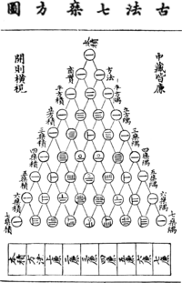
The fourth entry from the left in the second row from the bottom appears to be a typo (34 instead of 35, correctly given in the fifth entry in the same row).

The earliest explicit depictions of a triangle of binomial coefficients occur in the 10th century in commentaries on the Chandas Shastra, an ancient Indian book on Sanskrit prosody written by Pingala between the 5th century BC and 2nd century BC. While Pingala's work only survives in fragments, the commentator Halayudha, around 975, used the triangle to explain obscure references to Meru-prastaara, the "Staircase of Mount Meru". It was also realised that the shallow diagonals of the triangle sum to the Fibonacci numbers. The Indian mathematician Bhattotpala (c. 1068) later gives rows 0-16 of the triangle.

At around the same time, it was discussed in Persia by the mathematician Al-Karaji (953–1029) and the poet-astronomer-mathematician Omar Khayyám (1048-1131); thus the triangle is referred to as the "Khayyam triangle" in Iran. Several theorems related to the triangle were known, including the binomial theorem. It seems that Khayyam used a method of finding nth roots based on the binomial expansion, and therefore on the binomial coefficients.

In 13th century, Yang Hui (1238-1298) presented an arithmetic triangle, which was the same as Pascal's Triangle. Today, Pascal's triangle is called "Yang Hui's triangle" in China. In Italy, it is known as "Tartaglia's triangle", named for the Italian algebraist Niccolo Fontana Tartaglia who lived a century before Pascal.

In 1655, Blaise Pascal published its Traité du triangle arithmétique ("Treatise on arithmetical triangle"), wherein he collected several results then known about the triangle, and employed them to solve problems in probabilities. The triangle was later named after Pascal by Pierre Raymond de Montmort (1708) and Abraham de Moivre (1730).

After that, even if it was useful in many areas of mathematices, most research was done within its descendants, like probabilities and combinatorics.

Some Properties

Each term in the triangle is the sum of the two terms above it. For instance, $\scriptstyle 6=3+3$. The binomial coefficients relate to this construction by Pascal's rule, which states that if

${n \choose k}={\frac {n!}{k!(n-k)!}}$

is the kth binomial coefficient in the binomial expansion of $\scriptstyle (x+y)^{n}$, then

${n \choose k}={n-1 \choose k-1}+{n-1 \choose k}{\text{ with }}k,n\in \mathbb {N} ^{*}{\text{ and }}0\leq k\leq n$

By convention, the binomial coefficient $\scriptstyle {n \choose k}$ is set to zero if $\scriptstyle k$ is either less than zero or greater than $\scriptstyle n$.

To better understand some properties, the triangle is presented differently :

${\begin{array}{cccccccc}1&&&&&&&\\1&1&&&&&&\\1&2&1&&&&&\\1&3&3&1&&&&\\1&4&6&4&1&&&\\1&5&10&10&5&1&&\\1&6&15&20&15&6&1&\\1&7&21&35&35&21&7&1\\...&...&...&...&...&...&...&...\\\end{array}}$

Each coefficient is the sum of the coefficient exactly over it and its left neighbour. For instance, $\scriptstyle 3+3=6$. Let's call this rule the "addition rule".

Using this format, it is easy to apply an index to each row :

${\begin{array}{lcccccccc}0:&1&&&&&&&\\1:&1&1&&&&&&\\2:&1&2&1&&&&&\\3:&1&3&3&1&&&&\\4:&1&4&6&4&1&&&\\5:&1&5&10&10&5&1&&\\6:&1&6&15&20&15&6&1&\\7:&1&7&21&35&35&21&7&1\\...&...&...&...&...&...&...&...&...\\\end{array}}$

Starting the indices at zero facilitates many calculations.

The sum of any row is $\scriptstyle 2^{r}$, with $\scriptstyle r$ being the row index : $\scriptstyle 0,1,2,\ldots$ For instance, the sum of row 4 is $\scriptstyle 1+4+6+4+1=16=2^{4}$.

Since there is a formula for summing a row, then maybe there is one for a column ? It is the case. This time, we index the columns :

${\begin{array}{lcccccccc}&0&1&2&3&4&5&6&7\\0:&1&&&&&&&\\1:&1&1&&&&&&\\2:&1&2&1&&&&&\\3:&1&3&3&1&&&&\\4:&1&4&6&4&1&&&\\5:&1&5&10&10&5&1&&\\6:&1&6&15&20&15&6&1&\\7:&1&7&21&35&35&21&7&1\\...&...&...&...&...&...&...&...&...\\\end{array}}$

Anyone familiar with the factorial function can easily find the general formula. The sum of a column $\scriptstyle c$ ending at row $\scriptstyle r$ is

${\frac {(r+1)\times r\,\times \cdots \times (r-c+1)}{(c+1)!}}{\text{ with }}r,c\in \mathbb {N} ^{*}$.

There is another method to compute this sum, see .

Up until now, we added along the rows and the columns. We can add along the diagonals. Doing so from left to right and from bottom to top gives :

${\begin{array}{ccccccccccr}1&&&&&&&&&=&1\\1&&&&&&&&&=&1\\1&+&1&&&&&&&=&2\\1&+&2&&&&&&&=&3\\1&+&3&+&1&&&&&=&5\\1&+&4&+&3&&&&&=&8\\1&+&5&+&6&+&1&&&=&13\\1&+&6&+&10&+&4&+&1&=&21\\...&&&&&&&&&=&...\\\end{array}}$

The numbers on the right are the Fibonacci numbers.

One Row at a Time

We can build any row if we know the row before just by adding its terms two at a time. However, it is possible to build a row directly. We will build the row 4 in order to discover the rule. Each row starts with 1 :

${\begin{array}{lcccccc}4:&1&4&6&4&1&\\\end{array}}$

$1\times {\frac {4-0}{1+0}}=4~$

$4\times {\frac {4-1}{1+1}}=6~$

$6\times {\frac {4-2}{1+2}}=4~$

$4\times {\frac {4-3}{1+3}}=1~$

$1\times {\frac {4-4}{1+4}}=0~$

$\cdots ~$

${\binom {r}{c+1}}={\binom {r}{c}}\times {\frac {r-c}{1+c}}{\text{ with }}r,c\in \mathbb {N} ^{*}{\text{ and }}r\geq c~$

Once the row and the column indices are know, we can compute the neighbours, either right or left, of any term. Because it only applies to a row, we call it the "row rule".

Newton's Binomial Coefficients

Isaac Newton studied the triangle's properties and discovered two remarkable generalizations.

He extended the triangle along the negative axis. To better understand how he achieved this, let us write the triangle using another format :

${\begin{array}{lccccccccc}0:&1&0&0&0&0&0&0&0&...\\1:&1&1&0&0&0&0&0&0&...\\2:&1&2&1&0&0&0&0&0&...\\3:&1&3&3&1&0&0&0&0&...\\4:&1&4&6&4&1&0&0&0&...\\5:&1&5&10&10&5&1&0&0&...\\6:&1&6&15&20&15&6&1&0&...\\7:&1&7&21&35&35&21&7&1&...\\...&...&...&...&...&...&...&...&...&...\\\end{array}}$

Jacob Bernoulli is the "father" of this mathematical object named the "figurate number triangle". To ease the understanding in the following text, we will call it the "Bernoulli triangle", even is this matrix does not resemble a triangle anymore !

Using the row rule, let's compute the row -1 :

${\begin{array}{rrrrrrrr}-1:&1&-1&1&-1&1&-1&...\\0:&1&0&0&0&0&0&...\\1:&1&1&0&0&0&0&...\\2:&1&2&1&0&0&0&...\\3:&1&3&3&1&0&0&...\\4:&1&4&6&4&1&0&...\\5:&1&5&10&10&5&1&...\\...&...&...&...&...&...&...&...\\\end{array}}$

There is an infinity of $\scriptstyle 1$ and $\scriptstyle -1$. This is another hint that this object is a matrix. Each term in this row obeys the addition rule and the row rule. Some calculations should convince you.

We can further extend the triangle along the negative axis.

${\begin{array}{rrrrrrrrr}...&...&...&...&...&...&...&...&...\\-4:&1&-4&10&-20&35&-56&84&...\\-3:&1&-3&6&-10&15&-21&28&...\\-2:&1&-2&3&-4&5&-6&7&...\\-1:&1&-1&1&-1&1&-1&1&...\\0:&1&0&0&0&0&0&0&...\\1:&1&1&0&0&0&0&0&...\\2:&1&2&1&0&0&0&0&...\\3:&1&3&3&1&0&0&0&...\\4:&1&4&6&4&1&0&0&...\\5:&1&5&10&10&5&1&0&...\\...&...&...&...&...&...&...&...&...\\\end{array}}$

As we wrote earlier, Newton did not stop there. He asked himself if there were rows with fractional index, like $\scriptstyle {\frac {1}{2}}$. And the answer is yes !

In the preceding example, we computed the terms of row 4. Let's use that row again :

${\begin{array}{lcccccc}4:&1&4&6&4&1&\\\end{array}}$

$1\times {\frac {4-0}{1+0}}=4~$

$4\times {\frac {4-1}{1+1}}=6~$

$6\times {\frac {4-2}{1+2}}=4~$

$\cdots ~$

What is the first term of row $\scriptstyle {\frac {1}{2}}$? By definition, it is 1. What are the terms after that ? We will use the row rule to compute them !

$1\times {\frac {{\frac {1}{2}}-0}{1+0}}={\frac {1}{2}}~$

${\frac {1}{2}}\times {\frac {{\frac {1}{2}}-1}{1+1}}=-{\frac {1}{8}}~$

$-{\frac {1}{8}}\times {\frac {{\frac {1}{2}}-2}{1+2}}={\frac {1}{16}}~$

${\frac {1}{16}}\times {\frac {{\frac {1}{2}}-3}{1+3}}=-{\frac {5}{128}}~$

$\cdots ~$

No term goes to zero, even if each comes closer as it is further away from the first.

In the following augmented Bernoulli triangle, using the row rule, we added the rows $\scriptstyle {\frac {1}{2}}$ and $\scriptstyle {\frac {3}{2}}$ :

${\begin{array}{rrrrrrrrr}...&...&...&...&...&...&...&...&...\\-4:&1&-4&10&-20&35&-56&84&...\\-3:&1&-3&6&-10&15&-21&28&...\\-2:&1&-2&3&-4&5&-6&7&...\\-1:&1&-1&1&-1&1&-1&1&...\\0:&1&0&0&0&0&0&0&...\\{\frac {1}{2}}:&1&{\frac {1}{2}}&-{\frac {1}{8}}&{\frac {1}{16}}&-{\frac {5}{128}}&{\frac {7}{256}}&-{\frac {21}{1024}}&...\\1:&1&1&0&0&0&0&0&...\\{\frac {3}{2}}:&1&{\frac {3}{2}}&{\frac {3}{8}}&-{\frac {1}{16}}&{\frac {3}{128}}&-{\frac {3}{256}}&{\frac {7}{1024}}&...\\2:&1&2&1&0&0&0&0&...\\3:&1&3&3&1&0&0&0&...\\...&...&...&...&...&...&...&...&...\\\end{array}}$

Some calculations confirm that the addition rule works, as expected. After some tests, we see that it works only if the row indices have a difference of 1. For instance, we cannot easily build row 3.25 from row 3, but we can easily build row $\scriptstyle {\frac {3}{2}}$ from row $\scriptstyle {\frac {1}{2}}$. Up to a point, there are two matrices in the preceding Bernoulli triangle, one for the integers and one for the multiples of $\scriptstyle {\frac {1}{2}}$.

Newton's generalizations opened routes to areas not primarily connected to integers, namely numeric roots (like the square roots) and logarithms.

Computing a Root Square

Armed with the knowledge of the previous section, we are ready to compute the square root of a number.

We start with this equation :

$(x+y)^{2}=x^{2}+2xy+y^{2}~$,

If we replace $x~$ with 2 and $y~$ with 3, then we get

$(2+3)^{2}=2^{2}+2\times 2\times 3+3^{2}~$,

which is equal to 25, or $(2+3)^{2}=5^{2}~$. This is quite common knowledge, not to say boring.

Suppose we replace the exponent 2, an integer, by the exponent ${\frac {1}{2}}~$, a fraction. When the exponent value is 2, we get the square, when it is ${\frac {1}{2}}~$, we get the square root. This a rule of the exponentiation. Thus, we can use the triangle's terms to compute a square root.

This observation is technically correct, but there are some details that hugely simplify the calculations. If the exponent is a fraction, then $x~$ SHOULD be equal to 1 and, in this case, $y~$ MUST be equal to or less than 1. More preciseley, $|y|<1~$.

Let's compute $(2+3)^{\frac {1}{2}}~$, i.e. ${\sqrt {5}}~$.

$(2+3)^{\frac {1}{2}}=(4+1)^{\frac {1}{2}}=(4\times (1+{\frac {1}{4}}))^{\frac {1}{2}}=4^{\frac {1}{2}}\times (1+{\frac {1}{4}})^{\frac {1}{2}}=2\,(1+0.25)^{\frac {1}{2}}$

In the last parenthesis, $x~$ is equal to 1, and $|y|=0.25~$ is lower than 1. Here is how we proceeded. Compute the perfect square lower than $(2+3)~$, here it is 4. Change the sum within the parenthesis in order to display the perfect square. Get it outside the parenthesis, while applying the square root operation on both terms. Extract the square root from both, one requiring to use the binomial coefficients.

To compute the root square of the parenthesis, we use the row ${\frac {1}{2}}~$ in the triangle.

$(1+0.25)^{\frac {1}{2}}=1+{\frac {1}{2}}\times 0.25-{\frac {1}{8}}\times 0.25+{\frac {1}{16}}\times 0.25-{\frac {5}{128}}\times 0.25+{\frac {7}{256}}\times 0.25-{\frac {21}{1024}}\times 0.25\cdots$

$(1+0.25)^{\frac {1}{2}}=1+0.25\times ({\frac {1}{2}}-{\frac {1}{8}}+{\frac {1}{16}}-{\frac {5}{128}}+{\frac {7}{256}}-{\frac {21}{1024}}\cdots )$

$(1+0.25)^{\frac {1}{2}}\approx 1.1013183593$

Using six terms, the square root estimate of $(2+3)~$ is $2*1.1013183593=2.202636718~$. The square of this value is $4.8516085~$. Compared to the exact value, the error is close to 3%. Using more terms will sharpen the result.

We can compute any root with this method. However, it is not used in practice, since there are faster convergent methods, like the Newton-Raphson algorithm.

Computing the Logarithm of a Number

Starting with this equation :

$(x+y)^{2}=x^{2}+2xy+y^{2}~$,

we replace some terms within it :

$(1+z)^{2}=1^{2}+2\times 1\times z+z^{2}~$

$(1+z)^{2}=1+2z+z^{2}~$,

which is good for the square of $(1+z)~$. To compute the logarithm, we use the terms in row -1.

$(1+z)^{-1}=1-z+z^{2}-z^{3}+z^{4}-z^{5}+z^{6}+\cdots ~$

If we integrate both sides of the previous equation, we get the natural logarithm of a number :

$\ln {(1+z)}=z-{\frac {z^{2}}{2}}+{\frac {z^{3}}{3}}-{\frac {z^{4}}{4}}+{\frac {z^{5}}{5}}-{\frac {z^{6}}{6}}+{\frac {z^{7}}{7}}+\cdots {\text{ with }}z\in \mathbb {R} {\text{ and }}-1<z\leq 1~$

Normal Curve

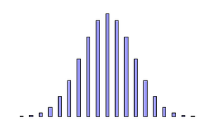
Pascal's triangle lends itself to graphical representation. If you draw an histogram of the 19Template:Th row coefficients, you would get something like the following picture.

Histogram of the row 19 within the Pascal's triangle

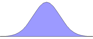
Suppose we compute the terms of the 1000Template:Th row in Pascal's triangle. If we divide each term by 2¹⁰⁰⁰ and consider each value as a point on a continuous curve, we would get the following curve.

The normal curve, a limit case of any row within the Pascal's Triangle, if the row has a sufficiently high order.

Gauss, the famous German mathematician, studied the normal curve. It is the commonest statistical law encountered in natural phenomenonsTemplate:,. For this reason, the properties of many statistical curves are compared to the normal curve properties. In its simplest form, its equation is $\scriptstyle P(z)=e^{-z^{2}/2}$.

Unexpected Relations

Odd numbers within a row

Each row of order $\scriptstyle 2^{n}-1,n\in \mathbb {N}$, only contains odd numbers. No other row has this property.

$\scriptstyle \pi$ and $\scriptstyle e$

We saw the normal curve, a way to represent the binomial coefficients as a continuous curve. In its simplest form, its equation $\scriptstyle P(z)=e^{-z^{2}/2}$ and the area under that curve is $\scriptstyle {\sqrt {2\pi }}$. The equation of this curve involves $\scriptstyle e$, while its area involves $\scriptstyle \pi$. How can this be possible, since the binomial coefficients are obtained by adding natural numbers, and we divided those coefficients by a power of 2 ?

Constructible polygons

Applying modulo 2 to every number in Pascal's triangle, we get

1

1 1

1 0 1

1 1 1 1

1 0 0 0 1

1 1 0 0 1 1

1 0 1 0 1 0 1

...

Viewing these ones and zeroes as binary digits, we get 1, 3, 5, 15, 17, 51,... in base ten. They are the number of sides found in constructible polygons with odd number of sides. This is true up to row 32.

Computing $\scriptstyle \pi$

We can compute $\scriptstyle \pi$ from the Pascal's triangle : $\scriptstyle {\frac {\binom {2n}{n}}{2^{2n}}}={\frac {1}{\sqrt {n\pi }}}$. For instance, $\scriptstyle {\frac {\binom {50}{25}}{2^{50}}}={\frac {1}{\sqrt {25\pi }}}$ outputs $\scriptstyle \pi =3.17316$. This formula is not used in practice since $\scriptstyle n$ must be very large to compute $\scriptstyle \pi$ to any decent precision.

Stacking marbles

If you stack marbles in the simplest 1D figure (along a line), then you arrange 1, 2, 3, 4,... marbles. If you stack marbles in the simplest 2D figure (triangle), then you arrange 1, 3, 6, 10,... marbles. If you stack marbles in the simplest 3D figure (a tetrahedron or 4-sided pyramid), then you arrange 1, 4, 10, 20,... marbles. If you stack marbles in the simplest 4D figure (a 4-simplex), then you arrange 1, 5, 15, 35,... marbles. And so on.

These numbers appear within the columns of the figurate number triangle, the column 1 contains the classic and basic counting numbers : 1, 2, 3, 4,... The column 2 contains the triangular numbers : 1, 3, 6, 10, 15, 21,... The column 3 contains the tetrahedral numbers : 1, 4, 10, 20, 35, 56,... The column 4 contains the pentatope numbers : 1, 5, 15, 35, 70, 126,... And so on.

Catalan numbers

The Pascal's triange hides the Catalan numbers.

1

1 1

1 2 1

1 3 3 1

1 4 6 4 1

1 5 10 10 5 1

1 6 15 20 15 6 1

1 7 21 35 35 21 7 1

1 8 28 56 70 56 28 8 1

...

Dividing the underlined numbers by 1, 2, 3, 4,..., we get 1, 1, 2, 5, 14,... The Catalan numbers appear in solutions of many geometrical problems. There is another way to compute these numbers : in the triangle, substract a neighbour from any underlined number.

There is a surprising way to compute them. Square the terms in each row and add them :

$\scriptstyle 1^{2}=1$

$\scriptstyle 1^{2}+1^{2}=2$

$\scriptstyle 1^{2}+2^{2}+1^{2}=6$

$\scriptstyle 1^{2}+3^{2}+3^{2}+1^{2}=20$

$\scriptstyle 1^{2}+4^{2}+6^{2}+4^{2}+1^{2}=70$

$\scriptstyle ...$

Geometric counting

Somebody found a strange property relating geometry to the numbers within the Pascal's triangle.

A dot has one vertex (1). A segment has two vertices and one line (2,1). A triangle has three vertices, three edges and one surface (3, 3, 1). A triangular pyramid has four vertices, six edges, four surfaces and one volume (4, 6, 4, 1). And so on. Thus, the element count of a minimal regular geometric object (build from regular shapes) in 1D, 2D, 3D, 4D, etc., is specified by a row in the Pascal's triangle.

Bernoulli numbers

Bernoulli numbers, named in honor of Jacob Bernoulli who studied them intensively, arise in a wide variety of analytical and combinatorial contexts. They are

$\scriptstyle B_{0}=1,\,B_{1}={\frac {1}{2}},\,B_{2}={\frac {1}{6}},\,B_{3}=B_{5}=B_{7}=...=0$

$\scriptstyle B_{4}=-{\frac {1}{30}},\,B_{6}={\frac {1}{42}},\,B_{8}=-{\frac {1}{30}},\,B_{10}={\frac {5}{66}},...$

Knowing that $\scriptstyle B_{0}$ and $\scriptstyle B_{1}$ are the two first terms of this series, we can compute all the terms : $<math>\scriptstyle B_{0}=1$, then B_0 = 1 </math>

$\scriptstyle B_{1}-B_{0}=-1/2$, then $\scriptstyle B_{1}=1/2$

$\scriptstyle B_{2}-2B_{1}+B_{0}=B_{2}$, then $\scriptstyle B_{1}=1/2$

$\scriptstyle B_{3}-3B_{2}+3B_{1}-B_{0}=B_{3}$, then $\scriptstyle B_{2}=1/6$

$\scriptstyle B_{4}-4B_{3}+6B_{2}-4B_{1}+B_{0}=B_{4}$, then $\scriptstyle B_{3}=0$

$\scriptstyle B_{5}-5B_{4}+10B_{3}-10B_{2}+5B_{1}-B_{0}=B_{5}$, then $\scriptstyle B_{4}=-1/30$

$\scriptstyle ...$

$\scriptstyle B_{1}$ is computed twice, but this arrangement clearly shows the binomial coefficients.